Conditional Formatting in Excel

gettingtheresometime

Can anyone help as I've been tearing my hair out for the last day trying to do something which (theoretically!) should be simple!

I've set up a spreadsheet for work that enables me to track invoices - so the columns include invoice date payment due date and a column whereby the age of the Invoice is calculated. The next two columns relate to the payment of the invoices - so a payment date and how much credit was taken. If there is an entry in the payment date, then the cell for the age of the invoice becomes empty.

What is giving me the grief is I want to conditionally format the first column that quotes the invoice number, but using the information as to the age of the invoice - so if it's over 30 days but under 60 it's filled with one colour but if it's over 60 days then I want it another colour. Sounds simple but it's beating me atm!

Any help would be appreciated

DE_612183

Conditional Formatting Based on Another Cell | Learn How to Apply? (educba.com)

DullGreyGuy

Assuming your "age" is in column D  and the first invoice is in A2 then you'd set a couple of rules for each colour with the rules being like...

=numbervalue($D2)>30 

The numbervalue function will deal with the cells you've blanked once paid presumably by having a formula outputting ""

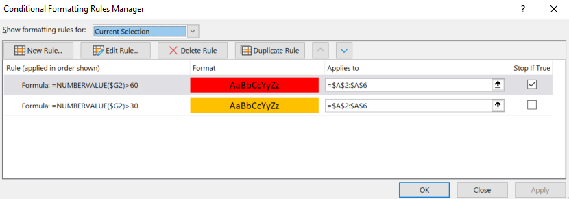
The rules need to be put in order of either high to low values in which case use the Stop if true checkbox or low to high in which case dont use them

gettingtheresometime

Thanks both for your replies but (and I'm now suspecting it's me!) they haven't helped.

The Invoice ref is in column A and the Invoice Age is in column G.

The formula I'm using in column G is if (H7="", datedif(D7, today(), "d")),"")) where Column D is the date of the Invoice & Column H is the payment date.

The rules I've used in Column A is G2>60 & and(G2>30,G2<60) .

DullGreyGuy

G7>60 will trigger on a case where H7 is blank because its not actually null but "" hence you need the numbervalue(G7) function as the "" will then be evaluated as 0

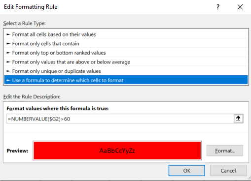
So in my example I created a rule on a range of cells in column A as:



Mine is G2 because the first cell in my range was A2... if yours is A7 then the formula would be G7

So with two rules on a top down basis they look like: