Spreadsheet formula for averages across irregular periods?

KingL2

Hi

Spreadsheet question:

I have some input data for a series of events that occur at irregular intervals

e.g. during hour=2, the real-world measured datum value is 323
then nothing happens until hour=9 when the real-world datum is 452

I want to 'spread' the value 323 over hours 0, 1 and 2 (i.e. calculate the average across those 3 hours (=323/3))

Then I want to spread the event that occurs at hour=9 (value=452) across the preceding 'zero value' hours (hours 3 to 9 (inclusive) i.e. 452/7

I can do it manually (Column D in the screenprint), but is there a way to put it in a formula that I can copy-paste down the sheet?

See the screencap of my manual version.

https://ibb.co/FbDzdZPS

Columns A & B are inputs from the real-world. Their values and time-of-occurance are irregular. I am trying to automate the calculation of Column D.

Stuff in italics is just commentary.

I'm using Libreoffice Calc v26.2. Have access to Excel 2013, if that helps.

MeteredOut

Not sure if you've tried, but this is the sort of thing AI is really good at answering.

Woodstok2000

CoPilot suggested using an 'if' and an xlookup formula to count the cells and work out the averages:

double_dutchy

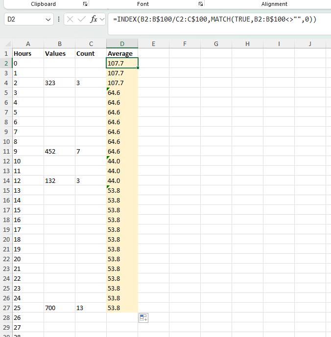
XLOOKUP isn't available in Excel 2013 but, without changing the data in column C, you can use this formula in D2 copied down to get the required results (assuming up to 100 rows of data, change as required)

=INDEX(B2:B$100/C2:C$100,MATCH(TRUE,B2:B$100<>"",0))

MyRealNameToo

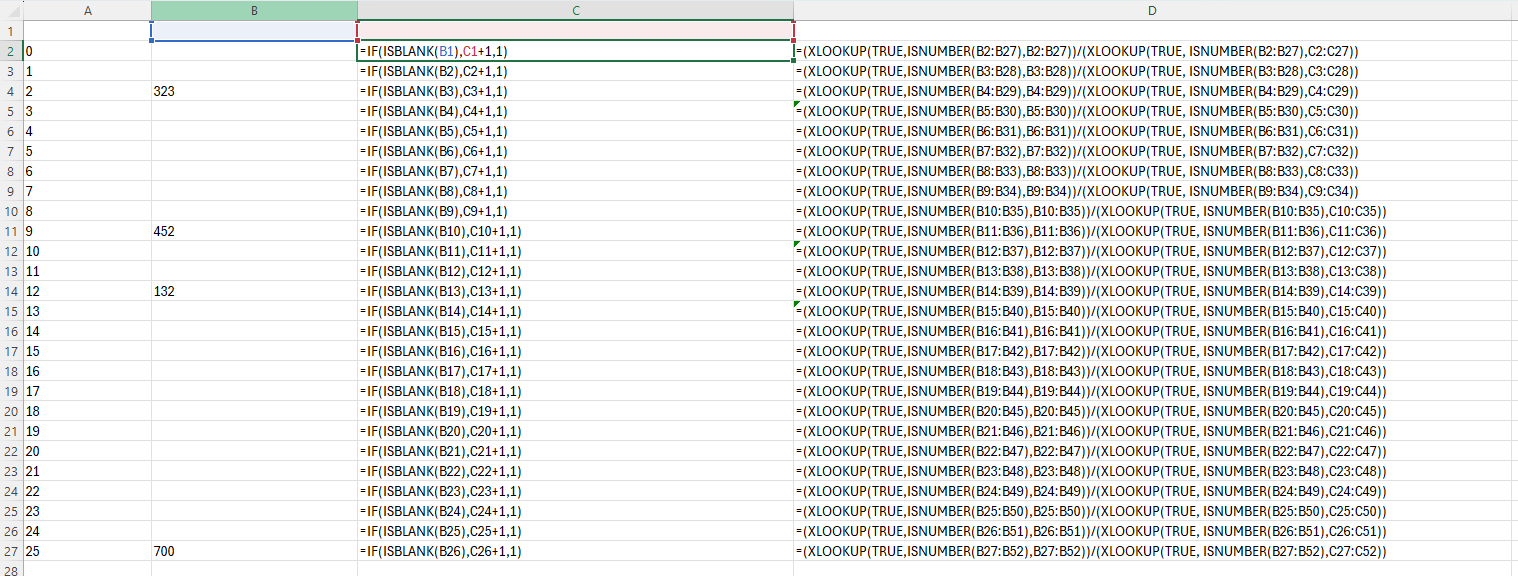
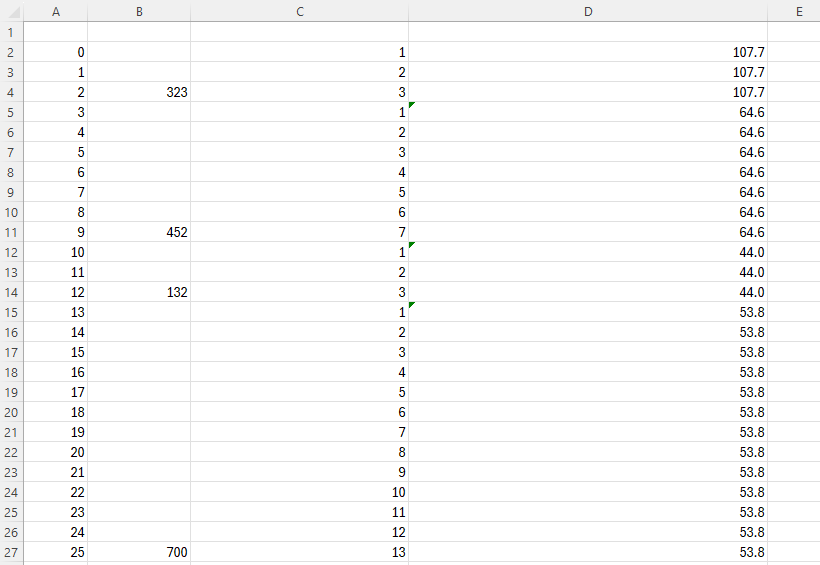
Personally would have a helper column in D staring at D2 of =COUNT(B$1:B1)+1

C then is =IF(SUMIF(D:D,D2,B:B)=0,"",SUMIF(D:D,D2,B:B)/COUNTIF(D:D,D2))

This deals with period 5 for which there is no measure

Vitor

AI says, put this in D2 and fill down. Change 1000 to a suitably large final row.

=IFERROR(INDEX($B:$B;ROW()-1+MATCH(1;INDEX(($B2:$B$1000<>"")*1;0);0))/(ROW()-1+MATCH(1;INDEX(($B2:$B$1000<>"")*1;0);0)-LOOKUP(2;1/($B$1:B1<>"");ROW($B$1:B1)));"")

It finds:

• the next non-blank measurement in column B
• the preceding measurement, or row 1 for the first period
• the number of rows between them, including the measurement hour

So it returns:

• hours 0–2: 323 / 3 = 107.7
• hours 3–9: 452 / 7 = 64.6
• hours 10–12: 132 / 3 = 44.0
• hours 13–25: 700 / 13 = 53.8

The IFERROR(...;"") leaves cells blank once there is no later measurement to allocate. This treats blank cells in column B as “no event”; a genuine measurement of zero still counts as an event.

double_dutchy

Hi Vitor,

AI isn't always the best at giving the most appropriate formulas in Excel. That much longer formula does the same as the one I suggested earlier (except for error checking), so my version with error checking would be:

=IFERROR(INDEX(B2:B$100/C2:C$100,MATCH(TRUE,B2:B$100<>"",0)),"")

This is an "array formula" in Excel 2013 so would need to be confirmed with CTRL+SHIFT+ENTER so that curly braces like { and } appear around the formula in the formula bar

To make it in to a "regular" formula, not requiring "array entry" you can add a couple of INDEX functions as follows:

=IFERROR(INDEX(INDEX(B2:B$100/C2:C$100,0),MATCH(TRUE,INDEX(B2:B$100<>"",0),0)),"")

Note that for a UK version of excel, comma separators would normally be used rather than semi-colons

Vitor

The formula I posted is in Libreoffice Calc syntax

double_dutchy

https://forums.moneysavingexpert.com/discussion/comment/82186941#Comment_82186941

Aah, sorry! assumed it was excel as that formula would also work in excel

KingL2

Awesome, thanks everyone. Vitor's one works perfectly in Libreoffice.

Out of interest, how would one phrase the question so that AI would understand it?

Vitor

I just posted your original text and image into ChatGPT