Emerging markets allocation (revisited)

OldScientist

A short while ago there was a thread here discussing Emerging Markets Allocation (https://forums.moneysavingexpert.com/discussion/6672348/emerging-markets-allocation ) that was closed at the request of the OP shortly before they left the forum.

I though that the research that was linked in the first post of that thread ( https://www.morganstanley.com/im/publication/insights/articles/article_howmuchtoown_us.pdf  ), which concluded that for US investors the allocation to EM should lie between 13% and 39% depending on the metric used, was interesting. So, since monthly return data for both EM and DM going back to the end of 1987 and 1969, respectively are freely available online (search ‘curvo MSCI world’ and ‘curvo MSCI emerging’) I thought it might be useful to dig a bit more into the conclusions made in that article.

To get an idea of the overall relative performance, the cumulative returns (i.e., index or growth chart) of EM and DM since the beginning of 1988 are plotted as a function of time in the top panel of the following figure, while the ratio of the cumulative returns, IEM/IDM (the so-called, ‘telltale chart’, e.g. see  https://johncbogle.com/speeches/JCB_Morningstar_6-02.pdf  ) is plotted in the lower panel. The telltale chart is useful since it allows the periods where EM outperformed (the gradient was positive) or underperformed (the gradient was negative) to be easily identified.

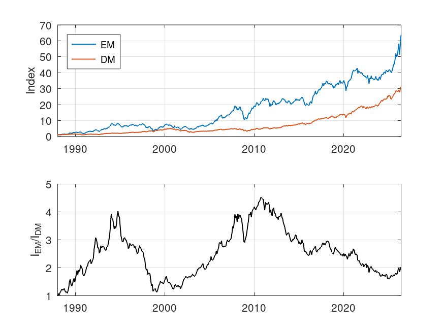
From the top panel, there are two things to notice, firstly that the returns for EM were higher over this 38 year period (also see table given below) and secondly, the volatility of the EM index was visibly higher. From the telltale chart in the lower panel, there were two periods where EM tended to outperform DM (1988 to 1995 and 2001 to 2011) and two periods where it tended to underperform (1995 to 1999 and 2011 to date).

The following table shows the annualised returns and standard deviation (in %) over the entire period. The annualised arithmetic mean were calculated using the formula 12*mean(monthly returns), the annualised geometric mean using product(monthly returns)^(12/N), where N is the number of monthly returns, and the annualised standard deviation using sqrt(12)*std(monthly returns).

	DM	EM
Arithmetic Mean	10.0	13.1
Geometric mean	9.4	11.4
Standard Deviation	14.1	21.1

Not surprisingly, the tabulated results confirm what was observed in the plot of cumulative returns, i.e., the annualised geometric return of EM was higher, by just under 2pp, but had a significantly larger standard deviation (i.e., volatility or risk).

For the active investor, predicting the periods of outperformance or underperformance would have been key to maximising returns (e.g., in the lower panel is the positive gradient over the last year or so indicative of a new, long, period of consistent outperformance or not?).

For the long-term buy and hold (i.e., passive) investor, the return data imply that holding some EM might have been useful (although less so in the last decade) in generating higher returns (but with more risk), but doesn’t really answer the question ‘how much?’. More on that in the next post.

aroominyork

If it's within your brief to look at equity income EM funds (eg DEM) in this analysis, I would find it interesting.

OldScientist

https://forums.moneysavingexpert.com/discussion/comment/82052782#Comment_82052782

As ever, it is a matter of finding (free!) data. I note that the US version of DEM (assuming that is the WisdomTree EM high dividend fund) has only been in existence since mid-2007 which only covers the last three years of outperformance by EM and the whole of the recent period of underperformance. Looking at the WisdomTree site, I note that in USD, DEM has grown from 10000 to 25926 since inception while MSCI EM and MSCI EM Value have grown 23361 and 23709, respectively. From this it seems that the returns over this limited period were fairly similar. I note that curvo does allow comparisons with the MSCI EMU high dividend yield index from 1995 onwards, but doesn't appear to have the raw data (again, there are periods of out and underperformance when compared with the vanilla EM index).

aroominyork

Thanks, OS. I am especially interested in volatility/risk. As is often the case, there is a potential trade-off with equity income = lower volatility = lower returns and I wonder if any numbers can be put to that?

Edit: Found it https://finance.yahoo.com/quote/DEM/risk

EthicsGradient

Curvo also calculate the Sharpe ratios for each, and say it's 0.61 for the MSCI World index, and 0.56 for their emerging markets measure, since the start of 1988:

Compare MSCI World vs Emerging markets · Backtest by Curvo

The Sharpe ratio of a portfolio measures its performance while taking account risk. If two portfolios have the same return but one of them has a lower risk, its Sharpe ratio will be higher. In other words, it measures the risk-adjusted return of a portfolio.

Sharpe ratio=𝐸⁢[𝑅𝑝−𝑅𝑓]/𝜎𝑝

where

𝑅𝑝 = return of the portfolio

𝑅𝑓 = risk-free return

𝐸⁢[𝑅𝑝 −𝑅𝑓] = annualised average monthly excess return

𝜎𝑝 = annualised standard deviation of the monthly excess returns

Backtest uses the Euribor 3 months rate as the risk-free rate

Bostonerimus1

https://forums.moneysavingexpert.com/discussion/comment/82053131#Comment_82053131

Any error bars on those ratios?

EthicsGradient

https://forums.moneysavingexpert.com/discussion/comment/82053508#Comment_82053508

No, but I'm not sure where you think the possible errors would creep in. They're calculated from actual values over the period. They're not predictions for the future.

easysaver

Interesting stuff OldScientist.

I've nothing constructive to add except perhaps that US investors will think differently regarding currency risk (I say differently because I don't understand the mechanisms!). I believe much of EM debt is in USD (although reducing in favour of Chinese denominated debt) but what about equity, I don't know?

I assume the index chart is linear? Logs would allow you to compare growths over different timescales (linear lends itself to full time period only unless your brain is wired differently!)

EthicsGradient

https://forums.moneysavingexpert.com/discussion/comment/82054543#Comment_82054543

If you go to the Curvo link I gave above, they plot the 2 indices together, and give you the choice of a log scale.

OldScientist

@EthicsGradient – I’m glad you mentioned risk, since that was where my next post was going. The Morgan Stanley paper (https://www.morganstanley.com/im/publication/insights/articles/article_howmuchtoown_us.pdf ) used the information ratio (IR) to compare the risk-adjusted returns of DM and EM. This is formulated in a similar way to the Sharp ratio, except that the risk-free return is replaced by a baseline return (in this case, the DM index). Goodwin (‘The Information Ratio’, 1998 which can be downloaded from https://tsgperformance.com/wp-content/uploads/2020/11/Goodwin-information-ratio.pdf) is a good introduction to this metric. High values of IR (typically a threshold of 0.5 is used) indicate that the portfolio (EM in this case) has a better risk-return than the baseline (DM in this case).

The following table shows the annualised mean excess return, MER, the annualised standard deviation of the excess return, SER and the information ratio, IR of the EM index using the DM index as a baseline for the arithmetic and geometric approaches for the periods 1988 to May 2026 and 1988 to end of 2020 (the latter period matches that used in the Morgan Stanley paper).

	MER (%)	SER (%)	IR
1988 to May 2026
Arithmetic	3.1	15.1	0.21
Geometric	1.9	15.1	0.12
1988 to end of 2020
Arithmetic	4.3	15.3	0.28
Geometric	2.9	15.3	0.19

According to the Morgan Stanley paper (Display 6), the IR of 100% EM index using the DM index as baseline lies between 0.48 and 0.49 for the period 1988 to the end of 2020 – this is much higher than the values I’ve calculated for the same period (i.e., 0.28 or 0.19 for arithmetic or geometric, respectively).

Given that IR=MER/SER, then in order to get the higher value of IR that Morgan Stanley present, either MER would need to be higher or SER lower. Since other calculations (e.g., at curvo) of the returns agree with mine it cannot be a discrepancy in MER. The SER for the two indices are 14.1% and 21.1% for DM and EM, respectively, so a value between the two for the excess return seems reasonable. To get the Morgan Stanley value of IR, SER would have to be about 8.9% or 6.0% (i.e. roughly half of the value I’ve calculated).

If the value I’ve calculated is correct, then this would imply that the results in Display 6 (and Display 7) of the Morgan Stanley paper are incorrect and that the optimum values of allocation to EM may also be in error. I’ve calculated the IR using two different methods (spreadsheet and programmed in octave) and while I don’t think I have made a mistake it would be useful if someone else on the board did the same set of calculations (the raw monthly index data are downloadable from curvo – a spreadsheet analysis of the arithmetic version of IR took me about 10 minutes) to check.

Notwithstanding the previous paragraph, one thing I was interested in was how IR varied with time. The following graph shows IR as a function of the start time for 5-year rolling periods for both arithmetic and geometric methods.

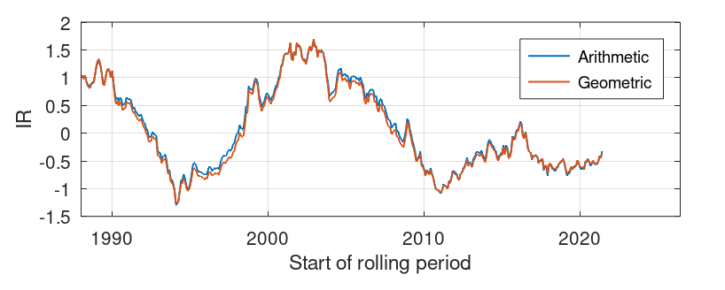
Two things can be noted. Firstly, IR was very variable and therefore strongly dependent on the start and end points chosen for calculation. A comparison of this graph with the telltale plot in the OP (i.e, the lower panel of the first figure) shows that, not surprisingly, IR was high for periods where EM outperformed and vice versa. Secondly, the difference between calculating IR using the arithmetic mean of excess returns and the geometric mean was small compared to the variation in IR with time, i.e. the simpler approach (arithmetic mean) is good enough.

OldScientist

https://forums.moneysavingexpert.com/discussion/comment/82053508#Comment_82053508

Annualised returns, and therefore Sharp ratios, are highly dependent on the chosen start and end times over which they are calculated. The values (i.e., 0.61 and 0.56) in the earlier post cover the period from 1988 (when MSCI started calculating the EM index) to end of May 2026. Changing the date range changes the ratio, for example, using the curvo link above, changing the start date to end of 1999 changes the Sharp ratios to 0.45 and 0.43 for DM and EM, respectively.

In that sense, there are uncertainties in the values (and future values are unknown).