Excel Pivot Table

sandy700

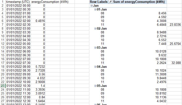
How do I sum every 5 rows without copy and pasting 90 times? the spreadsheet is 90 days.
I missed the column headers but the columns are A to G
Thanks

sandy700

and the sums are in column H =sum (G7:G4)

outtatune

Add another column called 'Row loop' or something like that, then =MOD(ROW(A1),5) and filling down will put 1,2,3,4,0,1,2,3,4,0,1 ... and so on down the column.

So in your pivot table filter or pivot on Row loop = 0.

Heedtheadvice

Twas a simple question but open to interpretation/confusion as to what you really want to do!

Is it get a total (sum) every five rows of the readings list....

Or is it sum every five rows of the pivot table, i.e. sum of daily readings?

...or something else?

The answer depends upon the clarification such as above method  (or other methods to do the same) or setting the pivot to give data summed by day....

sandy700

I want the sum of the values between 08:00 and 11:00 as my table, where I have done the first 3 sums.

It does not matter if it is done in the pivot table or in column B as long as I can show how much gas I have used every day between 08:00 and 11:00 hours.

As I said the only way I can figure out how to do it is to sum(G7:G4) then copy paste in column H every five rows for 90 times. 

Doshwaster

Using MOD is a  clever way, but if you want something simpler

<blank>
<blank>
<blank>
<blank>
=sum(of cells)

Select the cells in the block above then drag down the whole column so the pattern will repeat itself.

sandy700

if I enter 

=MOD(ROW(A1),5) 

in the column I have created (column H) it does not give any result, the formula just sits in the cell

outtatune

No, you create the row loop column in your source data, column C, not in the pivot table.

Heedtheadvice

I understand now thanks.

Many ways to do it;

one approach would to put a formula in column C (the next available to the consumption column) to test the time of day  meeting your spec under heading "TOD" or similar so you can add it into the pivot table and use it as a filter.

Such a formula in column c could be =AND( HOUR(A2) >= 8, HOUR(A2) <12) ...and copied all the way down of course.....

That would return True or False and including that column heading in the pivot table then is straight forward to sum days were that time period is True.

One could also use other formulae for other time periods if so desired combined with a lookup table for flexibility but that is beyond your question.