Any Google Sheets wizards that can help?

firsttimebuyer2013

Basically, I'm trying to get a sheet to do a sum, depending on what the drop down menu says.



The drop down menu will have about 4 options. The first one, if 'Cost' is selected, has to be C2-B2 witht the result in D2.

The second, with 'Profit', or two other choices under the dropdown (for example bonus, gift), just need to be whatever the value of C3 is to appear in D3.

Is this possible at all?

Thank you

cookie365

Simplest way is to use the IF function

http://spreadsheets.about.com/od/otherspreadsheets/qt/090808-google-spreadsheet-if-function.htm

firsttimebuyer2013

I had a look at that sheet but I'm still none the wiser. Can anyone help?

bluesnake

firsttimebuyer2013, the above link, look at row 5 in the example instead of "Yes", replace with "Cost", then do your sums

looks like you will need the OR function too to

A gift is a loss, so it is -1*C3 to appear in D3 ???

cookie365

I'm not going to second guess what the correct calculations should be.

If I've read the OP right then the calculation is that if the dropdown says 'Cost' it should be one calculation, and if it says anything else it should be another. In which case



[STRIKE]Otherwise, if there's a third calculation, 'nest' it where the final 'C2' bit is.[/STRIKE]

Edit: apparantly you can't nest IF statements on google sheets. That will make things interesting

bluesnake

cookie365 wrote: »

I'm not going to second guess what the correct calculations should be.

If I've read the OP right then the calculation is that if the dropdown says 'Cost' it should be one calculation, and if it says anything else it should be another. In which case



[STRIKE]Otherwise, if there's a third calculation, 'nest' it where the final 'C2' bit is.[/STRIKE]

Edit: apparantly you can't nest IF statements on google sheets. That will make things interesting

You can nest IF, but looks weird at first. D2 becomes

=if(A2="Cost",C2-B2, IF(A2="Gift",B2/-1, IF(A2="Profit",C2, IF(A2="Bonus","send money to bluesnake"))))

cookie365

bluesnake wrote: »

You can nest IF, but looks weird at first. D2 becomes

=if(A2="Cost",C2-B2, IF(A2="Gift",B2/-1, IF(A2="Profit",C2, IF(A2="Bonus","send money to bluesnake"))))

Ah yes, I found when I was in the nest clicking cells didn't copy them into the formula, so I assumed it wasn't possible. Just tried manually entering the nested formula and it works fine.


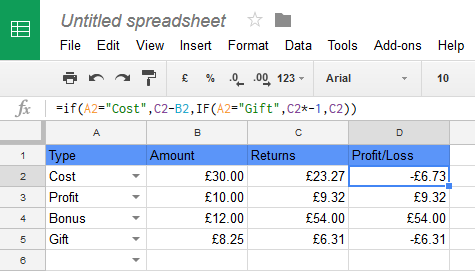
The way this formula works is it first looks at A2 and decides if it contains 'Cost'. If it does, it sets the cell to C2-B2 and stops. If it doesn't, it looks at the second IF statement.

It then looks to see if A2 contains 'Gift'. If it does, it sets the value to the negative flip of C2 and stops. If it doesn't, it sets the value to C2 and as there are no more nests the formula finishes.

firsttimebuyer2013

cookie365 wrote: »

Ah yes, I found when I was in the nest clicking cells didn't copy them into the formula, so I assumed it wasn't possible. Just tried manually entering the nested formula and it works fine.


The way this formula works is it first looks at A2 and decides if it contains 'Cost'. If it does, it sets the cell to C2-B2 and stops. If it doesn't, it looks at the second IF statement.

It then looks to see if A2 contains 'Gift'. If it does, it sets the value to the negative flip of C2 and stops. If it doesn't, it sets the value to C2 and as there are no more nests the formula finishes.

Thank you so much. Actually got it to work. Really appreciate that. :beer: